Dan Hicks - Difference-in-differences in R

This post recreates this post with proper formatting, syntax highlighting, etc.

library(tidyverse)

── Attaching core tidyverse packages ──────────────────────── tidyverse 2.0.0 ──
✔ dplyr     1.1.2     ✔ readr     2.1.4
✔ forcats   1.0.0     ✔ stringr   1.5.0
✔ ggplot2   3.4.2     ✔ tibble    3.2.1
✔ lubridate 1.9.2     ✔ tidyr     1.3.0
✔ purrr     1.0.2     
── Conflicts ────────────────────────────────────────── tidyverse_conflicts() ──
✖ dplyr::filter() masks stats::filter()
✖ dplyr::lag()    masks stats::lag()
ℹ Use the conflicted package (<http://conflicted.r-lib.org/>) to force all conflicts to become errors

library(skimr)

First we’ll load the data (download if necessary). I just started playing around with skimr::skim() to generate nice summaries. (digits doesn’t seem to do anything, though?)

data_file = '../_data/did_data.dta'
if (!file.exists(data_file)) {
    download.file(url = 'https://drive.google.com/uc?authuser=0&id=0B0iAUHM7ljQ1cUZvRWxjUmpfVXM&export=download', 
                  destfile = data_file)
}

dataf = haven::read_dta(data_file)
skim(dataf, work, year, children)

Data summary
Name	dataf
Number of rows	13746
Number of columns	11
_______________________
Column type frequency:
numeric	3
________________________
Group variables	None

Variable type: numeric

skim_variable	complete_rate	mean	sd	p0	p25	p50	p75	p100	hist
work	1	0.51	0.50	0	0	1	1	1	▇▁▁▁▇
year	1	1993.35	1.70	1991	1992	1993	1995	1996	▇▃▃▃▃
children	1	1.19	1.38	0	0	1	2	9	▇▃▁▁▁

Following the old post, we need to construct dummy variables for (a) before-and-after the EITC takes effect in 1994 and (b) the treatment group (1 or more children). We’ll keep these as logicals (rather than the numerics in the old post).

dataf = dataf %>%
    mutate(post93 = year >= 1994, 
           anykids = children >= 1)

The regression equation is

\[ work = \beta_0 + \delta_0 post93 + \beta_1 anykids + \delta_1 (anykids \times post93) + \varepsilon. \]

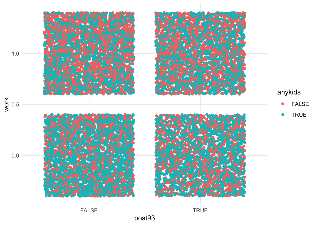
The “difference-in-differences coefficient” is \[\delta_1\], which indicates how the effect of kids changed after the EITC went into effect. Let’s take a second to plot this.

ggplot(dataf, aes(post93, work, color = anykids)) +
    geom_jitter() +
    theme_minimal()

Okay, so the scatterplot version, like, isn’t perspicuous. How about the un-dummied variables, and just the mean?

ggplot(dataf, aes(year, work, color = anykids)) +
    stat_summary(geom = 'line') +
    geom_vline(xintercept = 1994) +
    theme_minimal()

No summary function supplied, defaulting to `mean_se()`

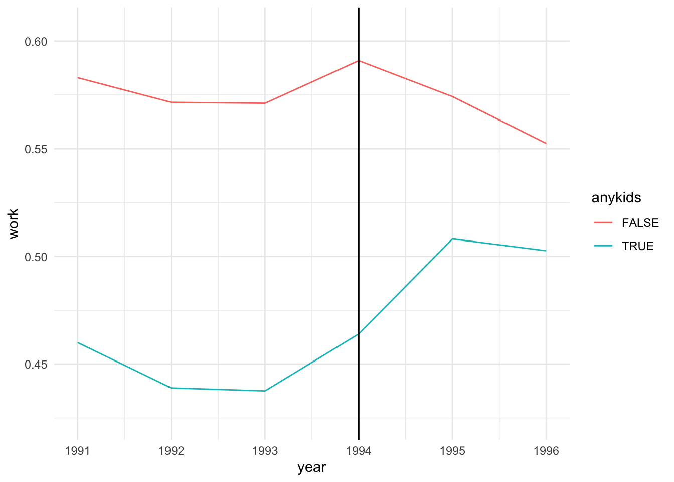
The parallel trends assumption looks good, at least qualitatively. (Remember this only applies prior to the intervention.) However, the parallel trends are nonlinear, which maybe is why the example uses the dummied variable.

Anyway, on to the regression. Which, hey, is a linear probability model because econometricians are funny like that.

model = lm(work ~ anykids*post93, data = dataf)
summary(model)


Call:
lm(formula = work ~ anykids * post93, data = dataf)

Residuals:
    Min      1Q  Median      3Q     Max 
-0.5755 -0.4908  0.4245  0.5092  0.5540 

Coefficients:
                        Estimate Std. Error t value Pr(>|t|)    
(Intercept)             0.575460   0.008845  65.060  < 2e-16 ***
anykidsTRUE            -0.129498   0.011676 -11.091  < 2e-16 ***
post93TRUE             -0.002074   0.012931  -0.160  0.87261    
anykidsTRUE:post93TRUE  0.046873   0.017158   2.732  0.00631 ** 
---
Signif. codes:  0 '***' 0.001 '**' 0.01 '*' 0.05 '.' 0.1 ' ' 1

Residual standard error: 0.4967 on 13742 degrees of freedom
Multiple R-squared:  0.0126,    Adjusted R-squared:  0.01238 
F-statistic: 58.45 on 3 and 13742 DF,  p-value: < 2.2e-16

This indicates that the EITC increased work (workforce participation? whether someone was employed?) by 5% among families with at least 1 child. In the second plot, the blue line goes from about 45% prior to 1994 to about 50% afterwards.