This morning I added a new feature to the blog posts: an R script that automatically generates and applies tags, allowing users to find old posts on (potentially, roughly) similar topics. Because of some difficulties setting up a chronological archive, I was worried old posts would be lost down the memory hole. This new feature should help prevent that.
My previous blogs had tags; you can see some of the remains of Tumblr’s tagging system at the bottom of many migrated posts. But the tags had to be added manually. This added a step to the publication process, and made me worried about inconsistent tags. What if I recently adopted a new tag that applied to some old posts? I’d have to scroll back through the archive to find them, which was both very tedious and prone to human error.
The new script solves these problems by automatically selecting tags and applying them across all posts at the same time. After writing a post, all I need to do is run a one-line command in the terminal. As a side effect, the tags will change, highlighting different arrays of topics as I add posts to the blog.
In the rest of this post, I want to explain the logic behind the tag selection process by walking through the code of the autotagging script. The post also includes a discussion of a metric I use for “high-information” terms, which I call \[n \Delta H\].
The script uses two R packages: tidyverse, a suite of packages of data wrangling; and tidytext, a text mining package designed for use with the tidyverse. After loading these packages, the rest of the following chunk loads the content of every post on the blog into a single dataframe structure.
library(tidyverse)
Warning: package 'tibble' was built under R version 4.5.2
Warning: package 'readr' was built under R version 4.5.2
Warning: package 'purrr' was built under R version 4.5.2
Warning: package 'dplyr' was built under R version 4.5.2
── Attaching core tidyverse packages ──────────────────────── tidyverse 2.0.0 ──
✔ dplyr     1.2.1     ✔ readr     2.2.0
✔ forcats   1.0.0     ✔ stringr   1.6.0
✔ ggplot2   3.5.2     ✔ tibble    3.3.1
✔ lubridate 1.9.4     ✔ tidyr     1.3.1
✔ purrr     1.2.2
── Conflicts ────────────────────────────────────────── tidyverse_conflicts() ──
✖ dplyr::filter() masks stats::filter()
✖ dplyr::lag()    masks stats::lag()
ℹ Use the conflicted package (<http://conflicted.r-lib.org/>) to force all conflicts to become errors
library(tidytext)post_folder =getwd() # Just `_posts/` in the actual scriptpost_files =list.files(post_folder, pattern ='\\.q?md') %>%file.path(post_folder, .)dataf =tibble(path = post_files) %>%mutate(post_id =row_number()) %>%rowwise() %>%mutate(raw_text =read_file(path)) %>%ungroup()str(dataf)
tibble [89 × 3] (S3: tbl_df/tbl/data.frame)
 $ path    : chr [1:89] "/Users/danhicks/Google Drive/Coding/website/posts/2012-03-14-friedersdorf-the-sex-friendly-case-against-free-bi"| __truncated__ "/Users/danhicks/Google Drive/Coding/website/posts/2012-03-14-friedersdorf-the-sex-friendly-case-against-free-bi"| __truncated__ "/Users/danhicks/Google Drive/Coding/website/posts/2012-04-21-the-agroecological-argument-for-eating-meat.md" "/Users/danhicks/Google Drive/Coding/website/posts/2012-05-23-fetishism-and-innate-differences.md" ...
 $ post_id : int [1:89] 1 2 3 4 5 6 7 8 9 10 ...
 $ raw_text: chr [1:89] "---\ntitle: \"Friedersdorf: The Sex-Friendly Case Against Free Birth Control, part I\"\ndate: \"2012-03-14\"\nc"| __truncated__ "---\nlayout: post\ntitle: \"Friedersdorf: The Sex-Friendly Case Against Free Birth Control, part II\"\ndate: \""| __truncated__ "---\nlayout: post\ntitle: \"The Agroecological Argument for Eating Meat\"\ndate: \"2012-04-21\"\ncategories: [d"| __truncated__ "---\nlayout: post\ntitle: \"Fetishism and Innate Differences\"\ndate: \"2012-05-23\"\n---\n\n\n(Going through m"| __truncated__ ...
Next we use tidytext to parse the text of each post into individual terms or tokens.
To develop tags, we want to identify “highly meaningful terms” across the cropus of parsed blog posts. In text mining, a measure called TF-IDF is frequently used for this task. TF-IDF is calculated for each term-document combination. The TF-IDF of term \[i\] in document \[j\] is - the number of times \[i\] occurs in \[j\] (the term frequency), divided by - the (log) number of documents in which \[i\] occurs at least once (the document frequency).
Intuitively, TF-IDF tries to identify words that are common in a particular document (high term frequency) but also only occur in a few documents (low document frequency). In English, words like “the” and “and” tend to have high term frequencies but also very high document frequencies, so their TF-IDF scores tend to be low. Misspelled words like “mipelled” have low document frequency, but also low term frequency, so again their TF-IDF scores tend to be low. Terms with a high TF-IDF should, the thought goes, be distinctive to a given document.
The problem with TF-IDF is that it’s difficult to make this intuitive account more precise. It can also be difficult to interpret, because the units are occurrences per log documents. Is 3 occurrences per log documents high or low? That depends on things like the number and length of documents in the corpus. In addition, TF-IDF is calculated for term-document pairs, not for individual terms. A word will have the same IDF value across the entire corpus, but will have different TF values as it occurs a different number of times across different documents.
For these reasons, in my text mining work I’ve switched to an information-based measure. To understand this one, note first that we have \[m=42\] blog posts. Suppose we draw one of these blog posts at random. The probability of drawing any given post is \[p(doc) = \frac{1}{m} = \frac{1}{42}\]. The entropy of this probability distribution tells us the number of binary bits (0s and 1s) we need to give a unique ID for each blog post.
\[ H = - \sum_{docs} p(doc) \log_2 p(docs) = - \sum_m \frac{1}{m} \log_2 \frac{1}{m} = log_2 m. \]
In the case of my blog before writing this post, the entropy is \[log_2 42 = 5.4\].
Now suppose that, after drawing a post at random, we draw a single word from the post at random (without peeking at exactly which post we’ve drawn). The probability that we’ve drawn any given post is now \[p(doc \mid word)\]. The information gain of the word is the difference between \[H\] up above and the entropy of this new distribution \[p(doc \mid word)\]:
\[\Delta H = H[p(doc)] - H[p(doc \mid word)].\]
We can think of \[\Delta H\] as the number of bits of information, relative to the full post ID, that we’ve gained from knowing the word. \[\Delta H\] corresponds to inverse document frequency (dividing by the document frequency) in TF-IDF: it tells us how unique that word is to each document. A term like “the” will tend to have \[\Delta H\] near 0 (it doesn’t give us any new information); a more distinctive term like “virtue” (only some of my posts are about virtue ethics) will have a relatively high \[\Delta\], perhaps 4 or even 5 (it tells us a lot about which particular posts we might have).
To calculate an overall score for each term, we multiply \[\Delta H\] by the (log) total times the term occurs across the entire corpus. Suppose “virtue” occurs 100 times across all blog posts, and has an information gain of 3 bits. Then we have \[\log_{10} n \times \Delta H = 2 \times 3 = 6\]. The units here are orders of magnitude-bits. An increase of 1 of these units means that a word occurs \[10\times\] as frequently or provides 1 added bit of information. I call the resulting measure \[n\Delta H\] (not writing the log for readability).
The following block calculates \[H\] for the distribution \[p(doc)\], as baseline, then calculates the information gain and \[n\Delta H\].
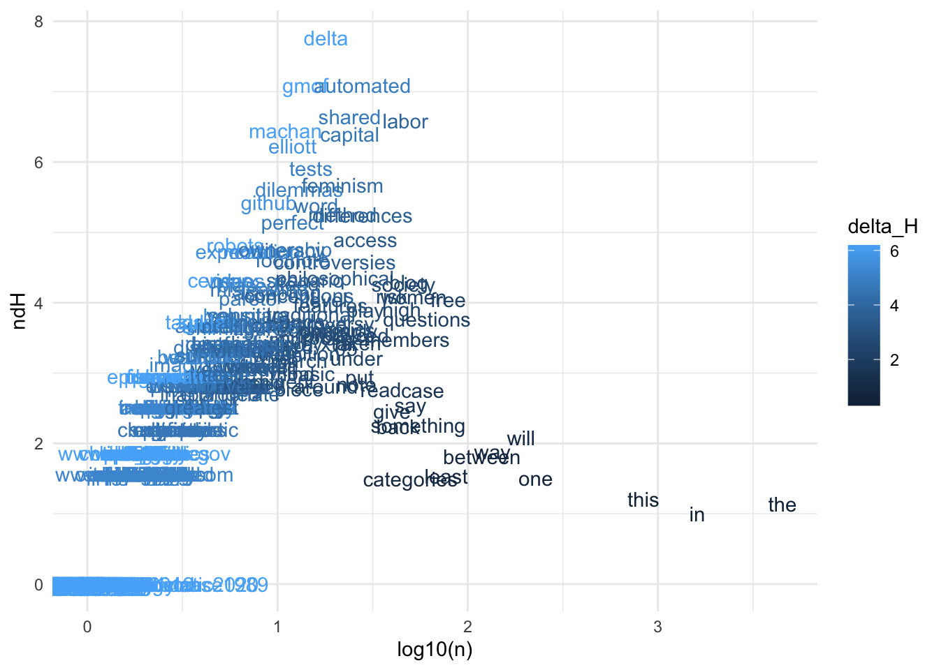
This next block isn’t included in the script; it generates a plot showing the distribution of \[n\Delta H\] scores for a sample of 500 terms. Each point represents a single term; the x-axis is the (log) number of total occurrences across the corpus, color indicates the information gain \[\Delta H\], and the y-axis is the overall \[n \Delta H\] score.
Informally, the \[n \Delta H\] score does a good job of identifying characteristic words for different kinds of posts, such as “data,” “developing,” and “feminism.”
The overall shape of the plot also shows how \[n \Delta H\] balances information gain and frequency. Some terms like “yourself” and “x’s” have a high information gain (more than 4 bits — remember that the maximum is about 5.4), but occur fewer than 10 times and so have a low \[n \Delta H\]. Extremely common terms (many more than 100 occurrences across a set of 42 posts) have very little information. The highest-scoring term, “market,” has both high information (4.3) and occurs 71 times.
All together, the \[n \Delta H\] score picks out a set of high-information, moderate-frequency terms in the middle of the plot, much like TF-IDF. In contrast with TF-IDF, it uses information theory for theoretical support and produces a relatively interpretable value.
The last step in the script is to select a vocabulary of terms to use as tags, identify them in the posts, and write the tags into the Markdown files.
To select the vocabulary, we simply take the terms with the highest \[n \Delta H\] scores. Because the blog is fairly small, it’s not unreasonable to take as many terms as there are blog posts (42 tags \[\to\] 42 tags). As the blog grows, I’ll probably want to trim this down to set a hard cap. Alternatively, I might want to select a number of tags such that each post has at least 1 tag and no post has more than, say, 5 tags. For now, though, I’ll just use the simpler logic of the top 42 terms.
vocab =top_n(info_df, nrow(dataf), ndH)
Then we’ll filter the list of tokens down to these tags, collapse the tags into a list, and convert the list into the string that will go in the header of the Markdown files.
`summarise()` has regrouped the output.
ℹ Summaries were computed grouped by path and post_id.
ℹ Output is grouped by path.
ℹ Use `summarise(.groups = "drop_last")` to silence this message.
ℹ Use `summarise(.by = c(path, post_id))` for per-operation grouping
  (`?dplyr::dplyr_by`) instead.
str(tags_df, max.level =1)
tibble [76 × 4] (S3: tbl_df/tbl/data.frame)
Finally we’ll write these files back to disk. Each post has a header section that looks something like this:
---title:"Post title goes here"style: postcategories:[monkey,zoo]---
We’ll separate this header section from the body by searching for the ---, add the tags, then put everything back together and write to disk. (Except we won’t actually write the results out to disk here.)
right_join(dataf, tags_df) %>%separate(raw_text, into =c('null', 'header', 'body'), sep ='---', extra ='merge') %>%## Remove old tagsmutate(header =str_replace(header, 'categories: \\[[^\\]]+\\]', '')) %>%mutate(combined =str_c('---', header, tags_str, '\n','---', body)) %>%# pull(combined) %>% {cat(.[[1]])}rowwise() #%>%